In part 1, I will discuss the invariance of QM under gauge transformations of the EM potential, and will address the matter of how to obtain the wave function for a quantum particle in a rotorless magnetic vector potential from that of a free particle as in the Wikipedia article cited in the enunciation of question. There, we will interpret the multivaluedness that appears in Wikipedia formula as a manifestation of the redundancy which is inherent of gauge invariance. In part 2, the Aharonov-Bohm (AB) effect will be derived from the path integral formalism. In part 3, I will discuss the electric version of the effect.
1. Let \(A^\mu=(\phi,\boldsymbol{A})\) be the EM potential. The action of a non-relativistic particle of mass \(m\) and charge \(e\) coupled to \(A^\mu\) is given by
\[S[\boldsymbol{x}(t)]=\int^{t_b}_{t_a}dt\big(\frac{1}{2}m \dot{\boldsymbol{x}}^2-e\phi(\boldsymbol{x}(t))+\frac{e}{c} \langle \dot{\boldsymbol{x}}, \boldsymbol{A} \rangle \big).\]
Let \(a=(t_a,\boldsymbol{x}_a)\) and \(b=(t_b,\boldsymbol{x}_b)\) be space-time events and \(K(b,a)=\langle t_b, \boldsymbol{x}_b|t_a,\boldsymbol{x}_b\rangle\) the propagator, which represents the transition amplitude for the particle to make the transition between states \(| a\rangle = |t_a,\boldsymbol{x}_a \rangle\) and \(|b \rangle=|t_b,\boldsymbol{x}_b \rangle\) (Heisenberg picture position eigenkets). In the path integral formalism,
\[K(b,a)=\int^b_a \mathcal{D}[\boldsymbol{x}(t)]e^\frac{iS[\boldsymbol{x}(t)]} {\hbar}
\\=\int^b_a \mathcal{D}[\boldsymbol{x}(t)]\mathrm{exp}\big(\frac{i} {\hbar} \int^{t_b}_{t_a}dt\big(\frac{1}{2}m \dot{\boldsymbol{x}}^2-e\phi(\boldsymbol{x}(t))+\frac{e}{c} \langle \dot{\boldsymbol{x}}, \boldsymbol{A} \rangle \big) \big).\]
A gauge transformation of the EM potential is performed by \(A^\mu \mapsto A'^\mu=A^\mu+\partial_\mu\Lambda\), where \(\Lambda \in C^\infty(\mathbb{R}^4)\). In vector calculus, this means \(\phi \mapsto\phi'=\phi-\frac{1}{c}\partial_t\Lambda\) and \(\boldsymbol{A}\mapsto\boldsymbol{A}'=\boldsymbol{A}+\vec{\nabla}\Lambda\). Applying this transformation to the action, \(S[\boldsymbol{x}(t)] \mapsto S'[\boldsymbol{x}(t)]\), one obtains that
\[S'[\boldsymbol{x}(t)]=S[\boldsymbol{x}(t)]+\frac{e}{c}\int^{t_b}_{t_a}dt\big(\partial_t \Lambda(\boldsymbol{x}(t))+\langle \dot{\boldsymbol{x}}, \vec{\nabla}\Lambda \rangle \big)
\\=S[\boldsymbol{x}(t)]+\frac{e}{c}\int^{t_b}_{t_a}dt \frac{d}{dt}\big(\Lambda(\boldsymbol{x}(t)) \big)
\\=S[\boldsymbol{x}(t)]+\frac{e}{c} \big[ \Lambda(\boldsymbol{x}(t_b))-\Lambda(\boldsymbol{x}(t_a)) \big].\]
Therefore, under a gauge transformation \(A^\mu \mapsto A'^\mu=A^\mu+\partial_\mu\Lambda\), the quantum mechanical propagator is transformed according to
\[K(b,a) \mapsto K'(b,a)=K(b,a) \mathrm{exp} \big( \frac{ie}{\hbar c} \big[ \Lambda(\boldsymbol{x}(t_b))-\Lambda(\boldsymbol{x}(t_a)) \big] \big).\]
Since the transition amplitude changed only by an overall complex phase, its squared modulus remains as before, and we conclude that QM is gauge invariant.
This result can be checked from the operator formalism as follows. We see from the above formula for the propagator change, \(K(b,a) \mapsto K'(b,a)\), that the gauge transformation of the EM potential is represented quantum mechanically by a unitary transformation \(\mathcal{G}(\Lambda)=e^{-ie\Lambda(\boldsymbol{x})/\hbar c}\) on the state space. This can be interpreted as a complex rotation of the (Schrodinger picture) position eigenkets, \(|\boldsymbol{x}\rangle\mapsto \mathcal{G}(\Lambda)|\boldsymbol{x}\rangle\). This being the case, if \(|\Psi\rangle\) represents the state of our system at initial time \(t_0\), we can associated a wave function \(\psi(t,\boldsymbol{x})=\langle\boldsymbol{x}|U(t,t_0)\Psi\rangle\) for all \(t \geq t_0\) (where \(U(t,t_0)\) is the time-evolution operator, as usual). The gauge transformation changes the wave function as
\[\psi(t,\boldsymbol{x})\mapsto\psi'(t,\boldsymbol{x})=\langle\boldsymbol{x}|\mathcal{G}(\Lambda)^+U(t,t_0)\Psi\rangle=\psi(t,\boldsymbol{x})e^{ie\Lambda({\boldsymbol{x}})}/\hbar c.\]
This gauge transformed wave function satisfy the associated gauge transformed Schrodinger equation, as can be checked from a direct calculation. (For details. cf. Sakurai section 2.6.) Moreover, the propagator written in the operator formalism changes as
\[K'(b,a)=\langle \boldsymbol{x}_b|\mathcal{G}(\Lambda)^+U(t_b,t_a)\mathcal{G}(\Lambda)|\boldsymbol{x}_a\rangle=K(a,b)e^{ie(\Lambda(\boldsymbol{x}_b)-\Lambda(\boldsymbol{x}_a))},\]
which is consistent with our path integral derivation.
Finally, as another viewpoint to understand the gauge invariance of QM, recall that from Ehrenfest theorem, we expect the average values \(<\boldsymbol{x}>\) and \(<\Pi>\) of the position \(\boldsymbol{x}\) and kinetic momentum operators \(\boldsymbol{\Pi}\) to satisfy the classical equations of motion, which do not involve the EM potential directly. So, these averages should be invariant under \(\mathcal{G}(\Lambda)\), as can be checked directly. (Recall that \(\boldsymbol{\Pi} = \boldsymbol{p}-e\boldsymbol{A}/c\), where \(\boldsymbol{p}\) is the canonical momentum, the one that satisfy the canonical commutation relation \([\boldsymbol{x},\boldsymbol{p}]=i \hbar\).)
Remark. From the above discussion, we can see that the Wikipedia article is right about the formula for the transformation of the wave function in the presence of a rotorless EM potential vector \(\vec{\nabla}\times \boldsymbol{A}=0\) in terms of the wave function for which the EM potential vanishes. Indeed, a rotorless potential vector can be introduced by a gauge transformation \(A^\mu \mapsto A'^\mu=A^\mu+\partial_\mu\Lambda\) for which \(\Lambda\) is time-independent, \(\partial_t \Lambda=0\). In this case, the new EM potential is given by \(\phi'=0\) and \(\boldsymbol{A}'=\vec{\nabla}\times\Lambda\), and the wave function becomes \(\psi'(t,\boldsymbol{x})=\psi(t,\boldsymbol{x})e^{ie\Lambda({\boldsymbol{x}})}/\hbar c.\) The multivaluedness of Wikipedia formula is actually a manifestation of the redundancy derived from gauge invariance. (Observe that our formula is obtained from that of Wikipedia by a sign reversion \(\Lambda \mapsto -\Lambda\), which is also allowed.)
2. Let us consider the typical Aharonov-Bohm (AB) experimental setting, where the potentials are such that \(\phi=0\) and \(\boldsymbol{A}\neq0\), the electric field strength vanishes everywhere, \(\boldsymbol{E}=0\), but the support of the magnetic field strength, \(\mathrm{supp}(\boldsymbol{B})\), is compact \(\subset\mathbb{R}^3\). The particle is created at the source, an event which we call \(a=(t_a,\boldsymbol{x}_a)\), and absorbed (or, as we say in QFT, destroyed) at the detector screen, an event which we call \(b=(t_b,\boldsymbol{x}_b)\). In Section 15 of Vol.2 of Feynman's lectures, now freely available here, this situation is illustrated in the following diagram:
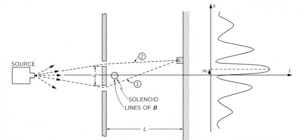
Let \(\boldsymbol{x}_1(t)\) and \(\boldsymbol{x}_2(t)\) denotes respectively the first and second paths. Returning to the path integral description, the sum over paths yields:
\[K(b,a)=\int^b_a \mathcal{D}[\boldsymbol{x}(t)]e^\frac{iS[\boldsymbol{x}(t)]} {\hbar}=\frac{1}{N}\big(e^{iS[\boldsymbol{x}_1(t)]/ \hbar]}+e^{iS[\boldsymbol{x}_2(t)]/ \hbar]} \big),\]
where \(N\) is a normalization constant (which appears naturally in Feynman's path integral measure). Writing the action for the particle motion as
\[S[\boldsymbol{x}(t)]=\int^{t_b}_{t_a}dt\big(\frac{1}{2}m \dot{\boldsymbol{x}}^2+\frac{e}{c} \langle \dot{\boldsymbol{x}}, \boldsymbol{A} \rangle \big)=S_0[\boldsymbol{x}(t)]+\frac{e}{c} \int^{t_b}_{t_a}dt\langle \dot{\boldsymbol{x}}, \boldsymbol{A} \rangle, \]
where \(S_0[\boldsymbol{x}(t)]=\int\frac{1}{2}m\dot{\boldsymbol{x}}(t)^2\) is the action for a free particle. Using the definition of path (in this case, line) integration, \(\int^{t_b}_{t_a}dt\langle \dot{\boldsymbol{x}}, \boldsymbol{A} \rangle=\int_{\boldsymbol{x}}\boldsymbol{A} \cdot d\boldsymbol{x}\), we finally have:
\[S[\boldsymbol{x}(t)]=S_0[\boldsymbol{x}(t)]+\frac{e}{c} \int_{\boldsymbol{x}}\boldsymbol{A} \cdot d\boldsymbol{x}.\]
Using this in the expression for the propagator, we deduce:
\[K(b,a)=\frac{e^{iS_0[\boldsymbol{x}_1(t)]/ \hbar]}}{N}e^{\frac{ie}{\hbar c} \int_{\boldsymbol{x}_1}\boldsymbol{A} \cdot d\boldsymbol{x}}+\frac{e^{iS_0[\boldsymbol{x}_2(t)]/ \hbar]}}{N}e^{\frac{ie}{\hbar c} \int_{\boldsymbol{x}_2}\boldsymbol{A} \cdot d\boldsymbol{x}}.\]
Letting \(K_i(b,a)=e^{iS_0[\boldsymbol{x}_i(t)]/ \hbar]}/N\) denote the free propagator associated with the path \(i\) and letting the unit complex phase \(e^{\frac{ie}{\hbar c} \int_{\boldsymbol{x}_1}\boldsymbol{A} \cdot d\boldsymbol{x}}\) in evidence, the expression for \(K(b,a)\) assumes the form:
\[K(b,a)=e^{\frac{ie}{\hbar c} \int_{\boldsymbol{x}_1}\boldsymbol{A} \cdot d\boldsymbol{x}} \big( K_1(b,a)+K_2(b,a)e^{\frac{ie}{\hbar c} \int_{\boldsymbol{x}_2-\boldsymbol{x}_1}\boldsymbol{A} \cdot d\boldsymbol{x}} \big).\]
Renormalizing the propagator as to eliminate the unit complex number in evidence and remembering from vector calculus that \(\int_{\boldsymbol{x}_2-\boldsymbol{x}_1}\boldsymbol{A} \cdot d\boldsymbol{x}=\int_\Omega\boldsymbol{B}\cdot d\boldsymbol{N}=\Phi\), where \(\partial \Omega=\boldsymbol{x}_2-\boldsymbol{x}_1\), we finally have the quantitative expression of AB effect:
\[K(b,a)=K_1(b,a)+K_2(b,a)e^{i\frac{e\Phi}{\hbar c}}.\]
Remark. The squared complex module of the propagator is:\[|K(b,a)|^2=|K_1(b,a)|^2+|K_2(b,a)|^2+2\big(\mathrm{Re}K^*_1(b,a)K_2(b,a)e^{i\delta}\big).\]
The third term accounts for the interference derived from the non-trivial EM potential, and the associated phase shift is \(\delta=e\Phi/\hbar c\). Observe that it is inaccurate to say (as it author of the question suggested) that the AB effect results in an overall phase shift, since this would have no effect upon the final measurement, namely, particle detection, because it would have no net effect on the complex module of the transition amplitude. What the AB effect really results in is a phase shift relative to the two amplitudes associated to each alternative path.
3. One might worry as the author of the question if there exists an electric analogue of the AB effect, and indeed, the answer is in the affirmative. Lets suppose that we have a not everywhere constant electric potential \(\phi\) and an everywhere vanishing magnetic vector potential, \(\boldsymbol{A}=0\). (We may in this case expect an effect already on the classical level, since spatial variation of \(\phi\) would imply in a nonzero electric field strength, \(\boldsymbol{E}=\vec{\nabla}\phi\neq0\).) Now the action reads
\[S[\boldsymbol{x}(t)]=S_0[\boldsymbol{x}(t)]-e\int^{t_b}_{t_b}\phi(\boldsymbol{x}(t))dt,\]
and the propagator for the transition from \(a\) to \(b\) now becomes
\[K(b,a)=\frac{e^{iS_0[\boldsymbol{x}_1(t)]/ \hbar]}}{N}e^{-\frac{ie}{\hbar} \int^{t_b}_{t_b}\phi(\boldsymbol{x}_1(t))dt}+\frac{e^{iS_0[\boldsymbol{x}_2(t)]/ \hbar]}}{N}e^{-\frac{ie}{\hbar} \int^{t_b}_{t_b}\phi(\boldsymbol{x}_2(t))dt}.\]
Lastly, rewriting the above equation in terms of \(K_i(b,a)=e^{iS_0[\boldsymbol{x}_i(t)]/ \hbar]}/N\) and renormalizing the probability amplitude, we deduce the analogous to the transition amplitude that appears in the AB effect in the presence of an electric potential:
\[K(b,a)=K_1(b,a)+K_2(b,a)e^{\frac{ie}{\hbar} \int^{t_b}_{t_b}[ \phi(\boldsymbol{x}_1(t))-\phi(\boldsymbol{x}_2(t))]dt}.\]
The resulting phase shift is therefore determined exclusively by the (time-integral) of the potential difference between the two alternative paths,
\[\Delta=\frac{e}{\hbar} \int^{t_b}_{t_b}[ \phi(\boldsymbol{x}_1(t))-\phi(\boldsymbol{x}_2(t))]dt.\]
If you imagine that capacitors (made of very large plates) are somehow placed along the two alternative paths, so that an approximately constant electric potential is held fixed along each path, say \(V_1\) and \(V_2\), the shift per unit time becomes \({\Delta}/T=e(V_1-V_2)/ \hbar\).
 Q&A (4831)